神经网络模型优化

★ 过拟合, 顾名思义 - 过度拟合训练集数据

在前面线性回归章节,我们就提及过过拟合问题.

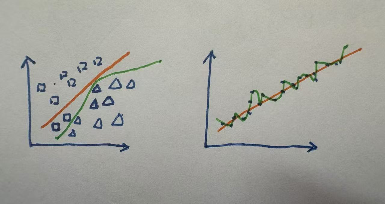
上图左侧是分类(xy轴都是特征),右侧是回归(x轴是特征,y轴是y_hat). 绿色-过拟合; 橙色-拟合.

# 原因1-模型过于复杂

模型过于复杂. 即过度拟合训练集数据, 造成过拟合

若模型在训练集上表现的很好,在验证集上表现的很差.说明过拟合了!

模型在train上学习到了一些跟分类任务无关的、不典型的特征
或者说train上的模型太复杂了,为了适应某些样本,但这样本可能是噪点、异常数据!
而在valid中,尽管valid的数据分布跟train上的数据相似,但valid上不具备这些不典型的特征,valid的acc就会比train的差很多!!
So,虽然复杂的深度学习更容易拟合训练集数据,但要尽量避免构建并训练过于复杂的模型..

假设这是有一个分类任务,数据集按照8:1:1的比例进行划分
在深度学习中,我们通常会把训练集进一步划分为训练集和验证集
> 其中训练集用于模型的训练 学习得到参数
> 验证集用于监督模型的训练效果
  即在每次模型训练后衡量模型的预测准确率,并与测试集中的准确率进行对比从而判断模型是否出现过拟合现象!!
> 测试集是模型从未见过的数据,体现的是模型的泛化能力

1
2
3
4
5
6

# 对微小变化很敏感

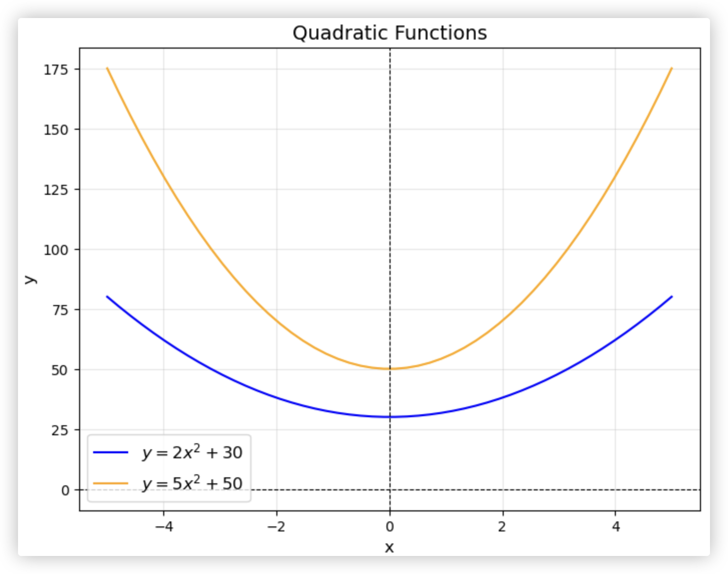
过度拟合训练集数据导致模型的数据对于输入数据的微笑变化很敏感. - 解决思路: 让w保持在一个尽可能小的值..

当模型的参数过大时,即使输入数据很小的变化,经过模型参数的计算也会对输出数据有很大的影响.

举个例子: 
- y_hat = 2x^2 + 30    w=2 b=30
- y_hat = 5x^2 + 50    w=5 b=50

> w大的,输入的x变化时,y_hat的波动比较大!! w大的,函数图像也会更抖一些!
  ★ ★ ★意味着,我们想让模型简单的话,就尽可能的让w保持在一个小的范围内!! （让x发生细微变化时,y_hat的值情绪别那么大,平稳些!）
> 权重w的值会影响函数抛物线的形状,而偏差的值只会影响图像在坐标系中的位置,不会对抛物线的形状产生任何影响.
  所以在后续对模型的过拟合的处理中,我们只会对模型的权重进行正则化!!

1
2
3
4
5
6
7
8

# T 解决方案: 正则化

前面我们说了,模型过于复杂,会导致模型的数据对于输入数据的微笑变化很敏感. - 过度依赖训练集,过拟合,泛化能力差.
我们提供了一个思路让模型尽可能的保持简单: 让w保持在一个尽可能小的值.

在该小节,我们用正则化来实现该思路!!

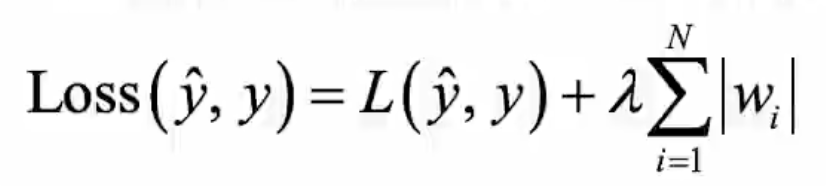
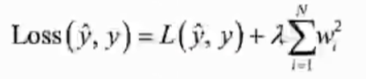
新loss(y,y_hat) = 旧loss(y,y_hat) + 正则项
1. 正则项满足 大于0
2. 让使新的loss(y,y_hat)尽可能的小,那么等式右边的两项都应该尽可能的小!!

L1 每个w尽可能等于0
L2 每个w尽可能的小

1
2
3
4
5
6

# L1正则

from keras.models import Sequential
from keras.layers import Dense
from keras.regularizers import l1
model = Sequential()
model.add(Dense(units=4, 
                activation='relu', 
                input_shape=(4,),
                kernel_regularizer=l1(0.01)))  # 0.01是拉不哒的值
model.add(Dense(units=1, 
                activation=None, 
                kernel_regularizer=l1(0.01)))

1
2
3
4
5
6
7
8
9
10
11

# L2正则

from keras.models import Sequential
from keras.layers import Dense
from keras.regularizers import l2
model = Sequential()
model.add(Dense(units=4, 
                activation='relu', 
                input_shape=(4,),
                kernel_regularizer=l2(0.01)))
model.add(Dense(units=1, 
                activation=None, 
                kernel_regularizer=l2(0.01)))

1
2
3
4
5
6
7
8
9
10
11

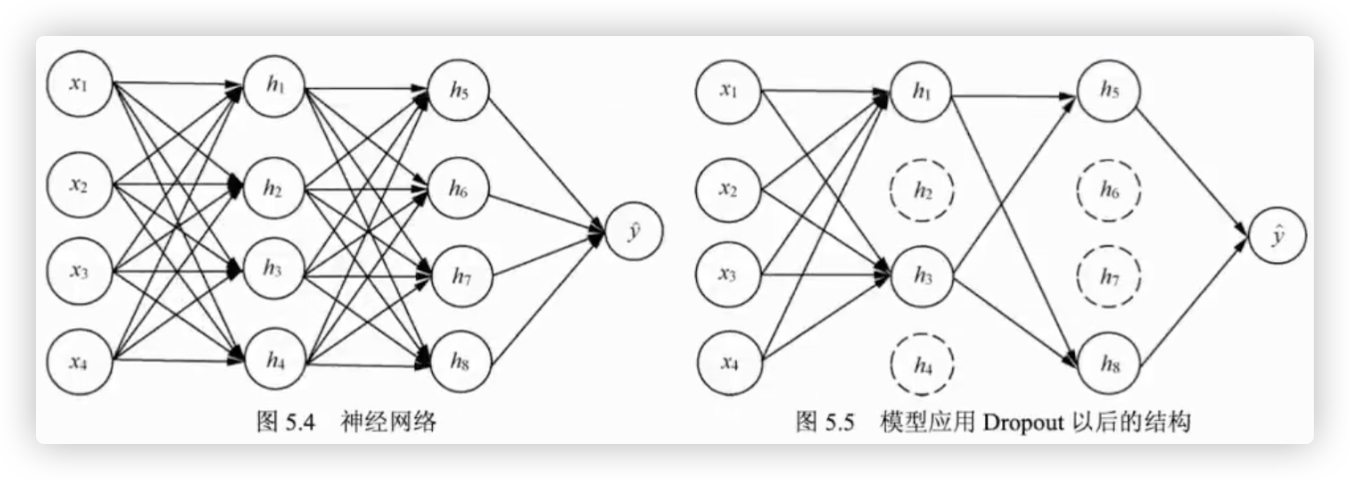
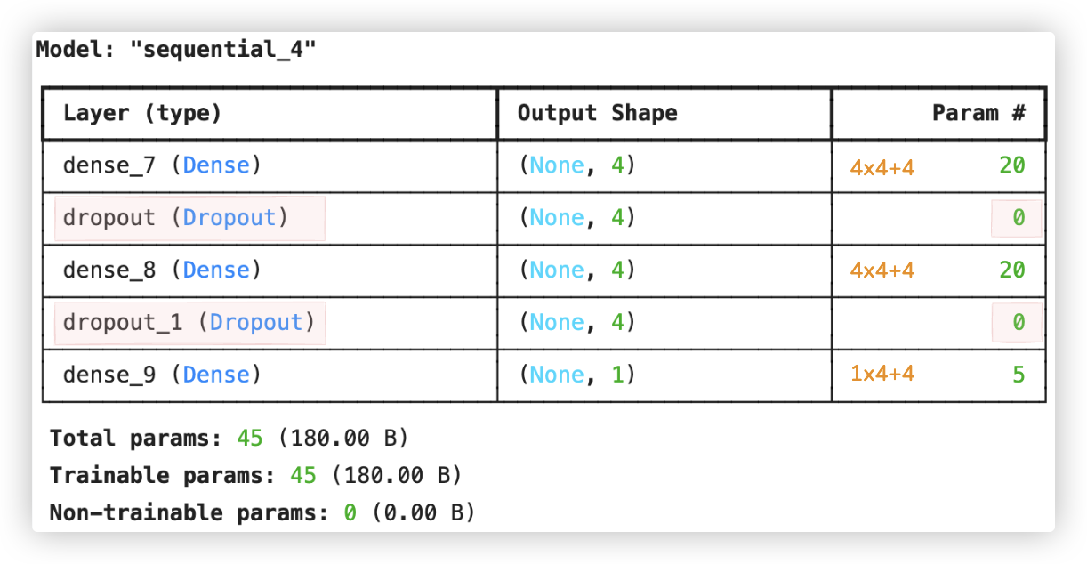
# T 解决方案: Droout应用

Dropout 的原理比较简单,在每一次模型训练时,按照一定的概率随机去掉神经网络模型中指定层的单元(节点)和与之相连接的权重.
这些被随机去掉的单元和与之相连接的权重不参与模型的训练, 只有与留下的单元相连接的权重才会得到更新.

from keras.models import Sequential
from keras.layers import Dense, Dropout

model = Sequential()
# 第一个中间层应用Dropout
model.add(Dense(units=4, activation='relu', input_shape=(4,)))
model.add(Dropout(rate=0.5))
# 第二个中间层应用Dropout
model.add(Dense(units=4, activation='relu'))
model.add(Dropout(rate=0.5))
# 输出层
model.add(Dense(units=1, activation='relu'))
model.summary()

1
2
3
4
5
6
7
8
9
10
11
12
13

# T 解决方案: 早停法

★ 在图中可以发现, 在模型训练过程中, 模型在验证集上的预测误差最小的时候, 是模型训练得最好的时候.

在这以前, 因为模型的预测误差还有下降空间, 所以这种现象称为欠拟合(underfitting).
模型没能够很好地拟合训练集中的数据.
在这之后, 因为模型过于拟合训练集数据, 进而失去了泛化能力, 所以称为过拟合.

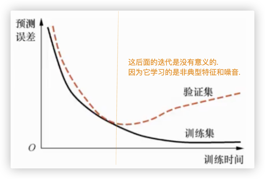
图中,由于迭代次数过多,造成了train loss持续下降,valid loss先下降后上升.

因此, 训练模型时如果在模型在验证集上的预测误差最小的时候停止训练, 既能够保证模型得到很好的训练, 又能够防止过拟合的发生.
这个方法就是早停（early stopping）法.

from sklearn.datasets import load_iris
from sklearn.model_selection import train_test_split
from keras.utils import to_categorical
# 加载鸢尾花数据集
iris = load_iris()
# 数据集中样本的特征值
X = iris.data
# 数据集中样本的标签值
y = iris.target
# 将数据集中的四分之三划分为训练集，四分之一划分为测试集
X_train, X_test, y_train, y_test = train_test_split(
    X, y, test_size=0.25, random_state=42
)
# 分别将训练集与测试集样本标签进行独热编码处理
y_train = to_categorical(y_train)
y_test = to_categorical(y_test)

from keras.models import Sequential
from keras.layers import Dense
model = Sequential()
model.add(Dense(50, input_shape=(4,), activation='relu'))
model.add(Dense(25, activation='relu'))
model.add(Dense(3, activation='softmax'))
model.compile(loss='categorical_crossentropy',
             optimizer='adam',
             metrics=['accuracy'])
model.summary()

from keras.callbacks import EarlyStopping
monitor = EarlyStopping(monitor='val_loss',   # 训练停止的衡量标准是验证集的损失值
                        min_delta=1e-3,       # 损失变化幅度0.001
                        patience=5,           # 耐心为连续5次
                        mode='auto',
                        verbose=1,            # 就在窗口输出日志的种类
                        restore_best_weights=True)

model.fit(X_train, 
          y_train, 
          validation_data=(X_test, y_test),  # 验证集使用的是测试集
          callbacks=[monitor],               # ☆使用早停法
          verbose=2,
          epochs=1000)  # 设置是1000次迭代,实则在100多次的时候就停止了!!

1
2
3
4
5
6
7
8
9
10
11
12
13
14
15
16
17
18
19
20
21
22
23
24
25
26
27
28
29
30
31
32
33
34
35
36
37
38
39
40
41
42

# 原因二-训练集样本数太少

数据集的不充足也会造成过拟合

想让模型在训练时探索特征与标签的关系,丢弃掉一部分非典型的特征,需要有充足的样本!
若训练集样本数太小,model就会过分的去利用train data.. 因为稀缺,所以极度压榨训练集.
像什么不典型特征,噪点,全利用了,,就过拟合了,它没有其它可以用的了啊!

# T 解决方案:增加样本

增加训练集中样本的个数是防止深度学习过拟合的最好方法之一 - data augmentation

在实际项目中,由于时间、经费、技术等的限制很难获得更多的数据来训练模型.
尽管如此, 还是可以通过现有的训练集来衍生出更多的数据样本.

对于图片数据,衍生出新的图片数据的一般方式为将图片旋转一定角度、改变图片的宽度与高度、缩放图片、改变图片亮度等.
通过这样的方法生成新的训练集来训练构建好的模型.
不仅可以有效地防止模型出现过拟合的现象,而且能够使训练的模型具有更好的鲁棒性

图片识别在深度学习之前是一个非常困难的任务! 图片翻转、图片亮度调整下,效果可能就不好了!
深度学习出现后,就会告诉模型,图片翻转、亮度改变啊,应该对标签毫无影响,模型会去抓主要特征去跟标签建立联系!

1
2

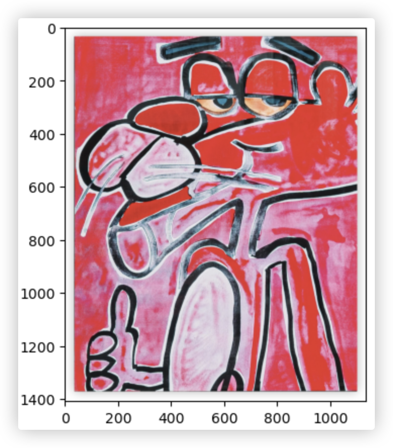
用代码实现下:

from keras.src.legacy.preprocessing.image import ImageDataGenerator
import numpy as np
import matplotlib.pyplot as plt

image_path = "wa.jpg"
image = plt.imread(image_path)
plt.imshow(image)   # 打印图片
print(image.shape)  # (1408, 1136, 3)

1
2
3
4
5
6
7
8

# 这些参数大多数都是范围
generator = ImageDataGenerator(rotation_range=10,        # 旋转
                               width_shift_range=0.1,    # 宽度
                               height_shift_range=0.1,   # 高度
                               shear_range=0.15,         # 图片剪切
                               zoom_range=0.1,           # 缩放
                               channel_shift_range=10,   # 三通道转换
                               brightness_range=(0.9, 0.7), # 亮度
                               horizontal_flip=True)        # 水平移动

# 因为我们通常会批量对多张图片进行 数据增强. 所以generator.flow()的api参数传的是4维数据
# 所以这里提前做下处理 3维变成4维度
image = np.expand_dims(image, 0)
print(image.shape)  # (1, 1408, 1136, 3)

# 衍生出10张图片
aug_iter = generator.flow(image)
aug_images = [next(aug_iter)[0] for i in range(10)]

# 展示下
def plots(ims, figsize=(12,6), rows=1):
    ims = np.array(ims).astype(np.uint8)
    fig = plt.figure(figsize=figsize)
    cols = len(ims) // rows if len(ims) % 2 == 0 else len(ims) // rows + 1
    for i in range(len(ims)):
        sp = fig.add_subplot(rows, cols, i + 1)
        sp.axis('Off')
        plt.imshow(ims[i])
        
plots(aug_images, figsize=(20,7), rows=2)

1
2
3
4
5
6
7
8
9
10
11
12
13
14
15
16
17
18
19
20
21
22
23
24
25
26
27
28
29
30

# 隐藏层数据批量标准化

加速收敛过程,减少训练时间 - 即减少模型迭代的次数,更快的得到最优参数!

在前面"全连接神经网络"博客的"梯度下降算法计算方式"小节中提到过,使用的训练集数据量.. (现目前所有示例都用的所有样本)
在这里,是对隐藏层的加权求和、经过激活函数后的向量进行标准化操作.. (看公式就明白了)

一般来说,深度学习模型会由多个隐藏层组成.
标准化训练集数据,也就是标准化模型输入层接收到的数据以加快模型的训练速度.
那么是不是标准化隐藏层接收到的数据也能加快模型的训练速度呢? 答案是肯定的.这就是批量标准化的由来.
因为深度学习模型在训练时一般会使用小批量的数据,如训练集中的16、32、64个样本数据.
所以在隐藏层每次也只能接收到小批量的数据,批量标准化就是标准化隐藏层接收到的小批量的数据.

1
2
3
4
5

以下是完整的对h1单元接收到的N个值进行批量标准化处理的过程.
同理,按照同样的方式,可以对隐藏层中其他单元接收到的值进行批量标准化. (标准化后数据的主要信息不会丢失,但会加快求导)

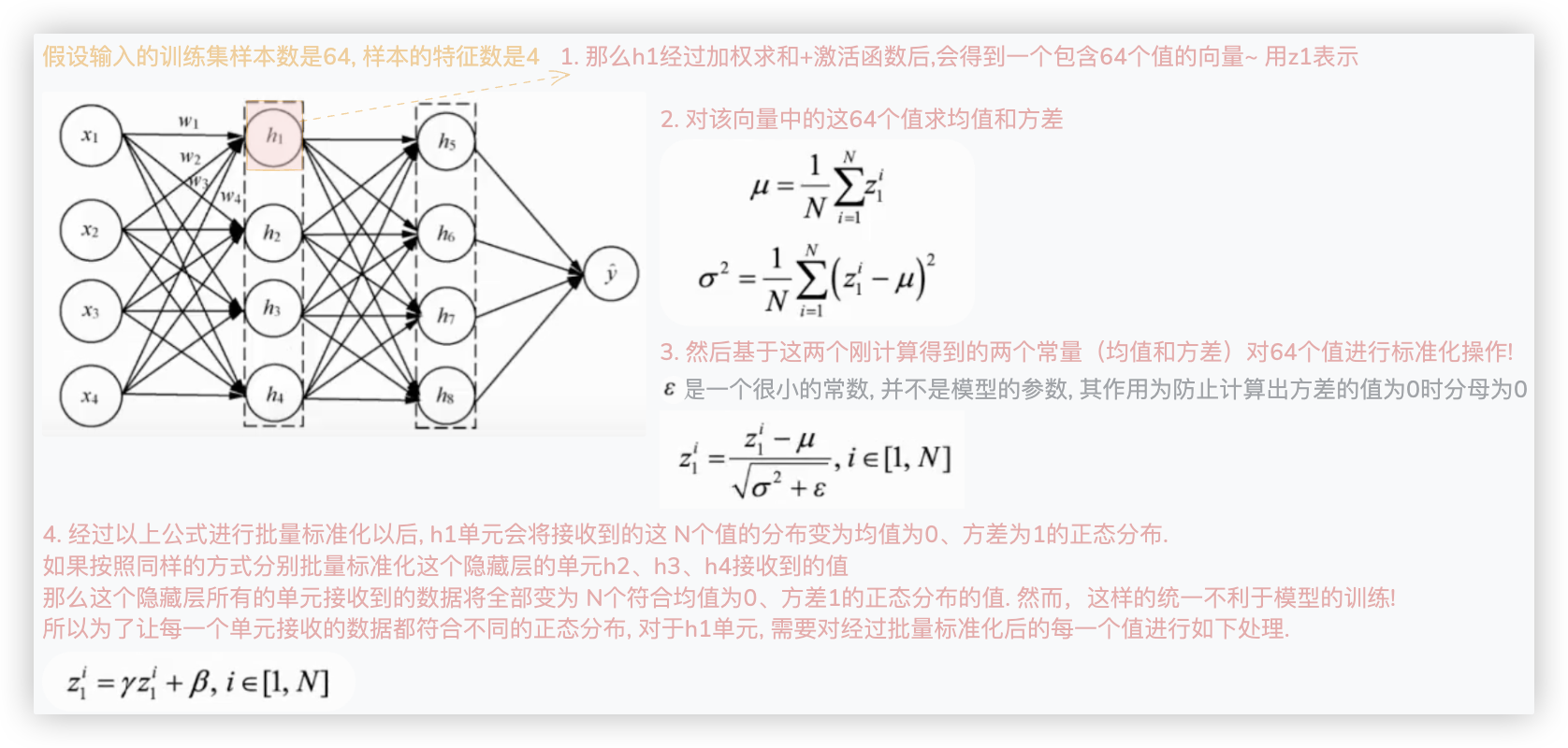
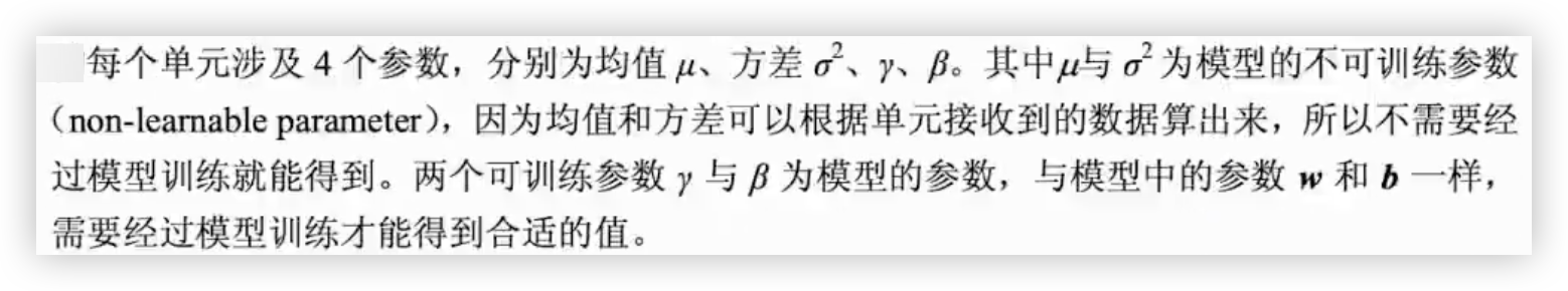
注意,在批量标准化的过程中,隐藏层的每个单元都涉及4个参数.

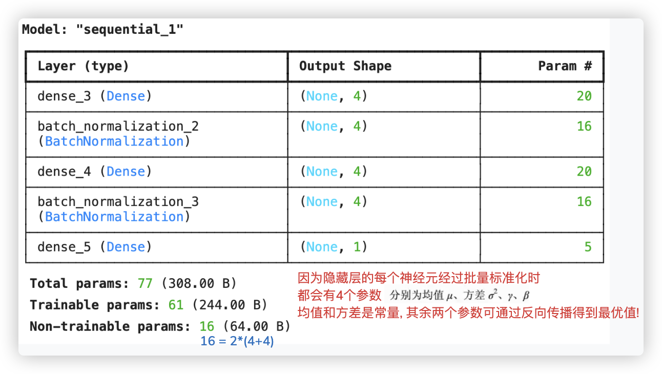
用代码来实现下:

from keras.models import Sequential
from keras.layers import Dense, BatchNormalization

model = Sequential()
# 第一个中间层应用批量标准化
model.add(Dense(units=4, activation='relu', input_shape=(4,)))
model.add(BatchNormalization())
# 第二个中间层应用批量标准化
model.add(Dense(units=4, activation='relu'))
model.add(BatchNormalization())
# 输出层
model.add(Dense(units=1, activation='relu'))
model.summary()

1
2
3
4
5
6
7
8
9
10
11
12
13

# CIFAR-10数据集分类项目实战

# 数据准备

from keras.datasets import cifar10
from keras.utils import to_categorical  # 独热编码
import numpy as np
import matplotlib.pyplot as plt

(X_train, y_train), (X_test, y_test) = cifar10.load_data()
y_train = to_categorical(y_train)
y_test = to_categorical(y_test)

X_train.shape  # (50000, 32, 32, 3) 5w张32x32的彩色图
y_train.shape  # (50000, 10)

1
2
3
4
5
6
7
8
9
10
11

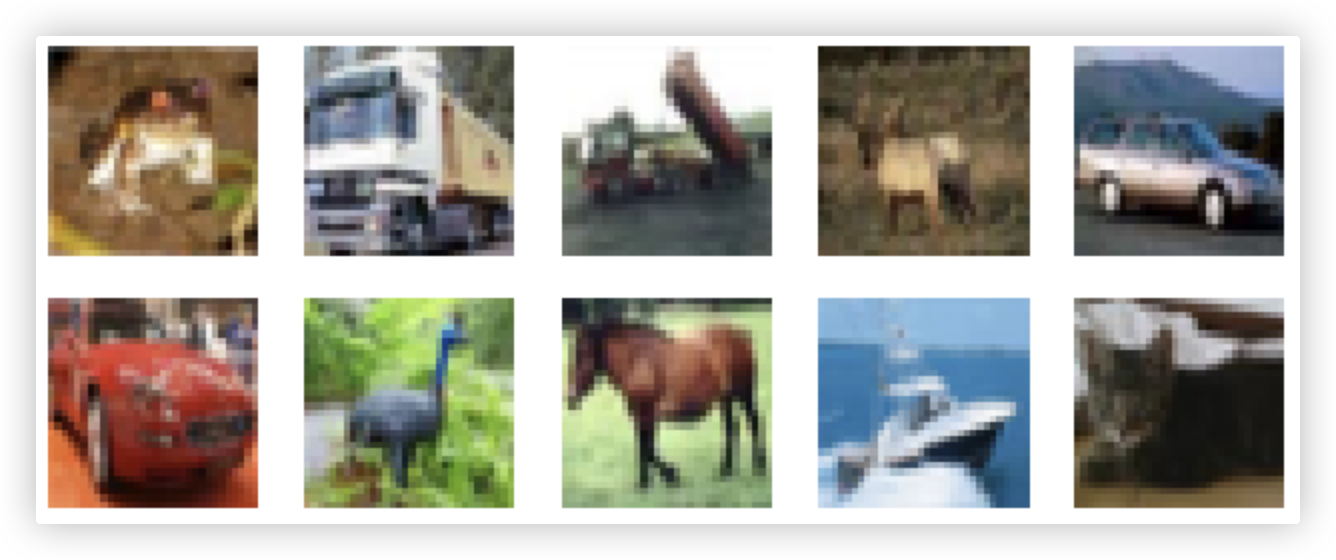
# 展示准备好的数据

def plots(ims, figsize=(12,6), rows=1):
    ims = np.array(ims).astype(np.uint8)
    fig = plt.figure(figsize=figsize)
    cols = len(ims) // rows if len(ims) % 2 == 0 else len(ims) // rows + 1
    for i in range(len(ims)):
        sp = fig.add_subplot(rows, cols, i + 1)
        sp.axis('Off')
        plt.imshow(ims[i])
        
plots(X_train[0: 10], figsize=(8, 3), rows=2)  # row的值应该是展示数量的公因数

1
2
3
4
5
6
7
8
9
10

# 构建模型结构

from keras.models import Sequential
from keras.layers import Flatten, Dense
from keras.layers import Dropout, BatchNormalization
from keras.optimizers import RMSprop

model = Sequential()
# 模型的输入层
model.add(Flatten(input_shape=(32, 32, 3)))  # 每个样本(1,32,32,3)展平成(1,32*32*3)
# 第一个中间层
model.add(Dense(256, activation='relu'))
model.add(BatchNormalization())  # 隐藏层数据批量标准化
model.add(Dropout(rate=0.2))     # dropout防止过拟合
# 第二个中间层
model.add(Dense(256, activation='relu'))
model.add(BatchNormalization())
model.add(Dropout(rate=0.2))
# 第三个中间层
model.add(Dense(128, activation='relu'))
model.add(BatchNormalization())
model.add(Dropout(rate=0.2))
# 第四个中间层
model.add(Dense(128, activation='relu'))
model.add(BatchNormalization())
model.add(Dropout(rate=0.2))
# 模型的输入层
model.add(Dense(10, activation='softmax'))
# 指定优化器、loss、评估
model.compile(optimizer=RMSprop(),
              loss='categorical_crossentropy',
              metrics=['accuracy'])

1
2
3
4
5
6
7
8
9
10
11
12
13
14
15
16
17
18
19
20
21
22
23
24
25
26
27
28
29
30

# 数据增强 - 增加样本

from keras.src.legacy.preprocessing.image import ImageDataGenerator

generator = ImageDataGenerator(
    featurewise_center=True,
    featurewise_std_normalization=True,
    rotation_range=20,
    width_shift_range=0.2,
    height_shift_range=0.2,
    horizontal_flip=True)
generator.fit(X_train)

1
2
3
4
5
6
7
8
9
10

# 模型训练

model.fit(
    generator.flow(X_train, y_train, batch_size=64),  # 不纠结这里数据增强咋搞的,简单理解成设置了batch_size=64
    # steps_per_epoch=1500,  # 若不设定,每个迭代默认的BP次数是 训练样本数 / batch_size
    epochs=5)

1
2
3
4

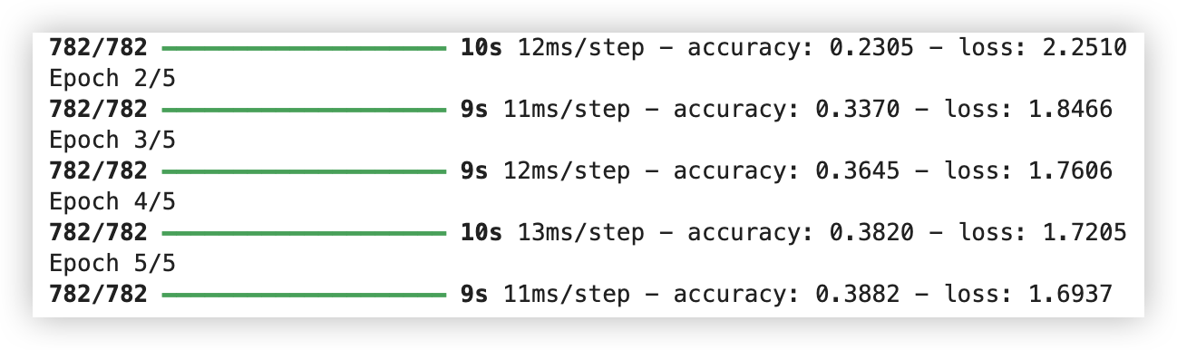
50000/64=781.25

# 模型保存和加载

"""
模型保存
"""
model.save("model.h5")  # 包含模型结构和参数 有多种后缀 .h5、.keras、.tf

json_string = model.to_json()  # 模型的结构
model.save_weights("model.weights.h5")  # 模型的参数


"""
模型加载
"""
from keras.models import load_model
model = load_model("model.h5")

from keras.models import model_from_json
model_architecture = model_from_json(json_string)
# 在模型的结构中加入模型参数
model_architecture.load_weights("model.weights.h5")

1
2
3
4
5
6
7
8
9
10
11
12
13
14
15
16
17
18
19

← 全连接神经网络卷积神经网络→